It’s A Small Cluster After All


Recently, DomainTools presented a webinar on using Data Science techniques to assist a Threat Intelligence investigation into the Disneyland Team. We showed how clustering algorithms and text processing techniques can group domains together into their assumed impersonation target, and also how to cluster subdomains together by their behavior. Today we are releasing our research notes from that investigation. You can download them from GitHub here.
The Jupyter notebooks we are releasing today have a fair amount of comments in them that should be a starting point to understanding what we did. If you’re interested in a more in-depth discussion of what’s happening in there, read on – we’ve linked each section title to the notebook that it talks about so you can follow along.
Otherwise, if you’re more of the dive-head-first-into-a-challenge type, click that github link above, and have fun!
What’s the Big Idea?
One of our Principal Solutions Architects (who spends a considerable amount of time doing research), Clay Blankinship, read Brian Krebs and Hold Security’s article on the Disneyland team, and was curious to see if he could find more information in DomainTools data. He succeeded. In fact, starting from 14 domains, he finished with nearly 500. When he shared that with the DomainTools Research team, we wanted to see if we could help & if we could pull any useful information out of that pile of domains.
Our first step was to download data out of Iris Investigate, which gave us a big list of everything we had on those domains (Whois info, IP addresses, nameservers, etc). For the most part, we’re only using the domain name itself from that download, but the create date will be useful later.
Let’s look at a few of the domain names:
țanqerine[.]com
țanqerlne[.]com
șẹb-lv[.]com
șẹb[.]com
ụșbamh[.]com
ụșbamk[.]com
There’s a lot going on here. As mentioned by Brian Krebs, they look like they’re impersonating bank domains, but with a few twists: there’s a lot of what appear to be homoglyph attacks, as well as typo attacks. So what are those?
Homoglyph attacks are a way to trick users with impersonations of common brands/websites by using characters from Unicode that resemble other letters. For example, the
e
in what looks like “
seb[.]com
” above is actually
ẹ
(note the dot under the e). Users who are just glancing at their URL bar may not notice the difference between
google.com
and
googlẹ.com
, but from the point of the computer (and the Internet), those are different domains. Such domains are often encoded using a technique called punycode encoding. The punycode representation of
googlẹ.com
(with the dotted-e) is actually
xn--googl-r51b.com
.
Typo attacks are similar, though they don’t rely on Unicode. Instead they use visually-similar letters or sets of letters. For example, g and q can be mistaken for each other by a quick-reading user, as can
m
and
n
. You see both of those above. You may also see more complex substitutions such as
rn
for
m
. As with the homoglyphs above, they may look visually similar to a user, but to the Internet,
rnicrosoft.com
is a distinct and different domain than
microsoft.com
.
Act 1, DomainTools 0
First we applied the clustering approach from an earlier webinar Reel Big Phish: Hunting For Badness in a Sea of Noise. This approach was straightforward: use Zipf’s law to split each domain into a set of words (see this blog post for details), then group the small sets of words together by how many words each set had in common.
First, we removed homoglyphs to allow the words to cluster together. For this round of the investigation, we mapped out all the Unicode homoglyph characters manually and replaced them with their ASCII equivalents. That won’t scale to the more general case of all possible homoglyphs, but it was good enough for our use case here.
Once that was done, it was on to clustering the domain “documents” together with DBSCAN.
Sidebar – Clustering
We did the clustering with an algorithm called DBSCAN. Why DBSCAN? There are two main ways we felt we could approach this clustering, K-Means and DBSCAN. K-Means is a way of grouping things together by first laying out the entries you’re trying to cluster in some coordinate space, then measuring how “close” they are to a chosen point in that space. You pick a number of “centroids” (or centers of clusters), toss them randomly across the space, measure which entries end up closest to which centroid, then adjust the locations of each centroid to minimize the distance to the elements in its cluster…and repeat that process until things stop moving around. That works well for things that are easily numericalized, but does require you to manually pick “k,” the number of clusters or centroids you’re working with.
DBSCAN comes at the problem from another direction. It instead looks at areas of density in the coordinate space, and asks you to specify how far apart is “too far” for two things to be in the same cluster. It then identifies the areas of high density where everything inside the minimum distance is in the same cluster. This has the side-effect that some entries that are far from anything else (in a low-density area) might not be in any cluster. Like k-Means, you do have to manually choose the max distance, called “epsilon,” and you can also set a variable which specifies how many entries there must be at a minimum for there to be a real cluster. But, DBSCAN does not require you to specify how many clusters there should be. One other side-effect of DBSCAN is that it will have a “none-of-the-above” cluster, which is where the things that happened to fall in the low-density areas are put. Things in the none-of-the-above cluster aren’t necessarily similar to each other, it’s that they’re not close enough to *anything*.
In general K-Means works well for sparse data and for data that is somewhat uniformly distant from positions in space. DBSCAN works better for data that can be sparse in areas and dense in others. We felt like the distribution of words was likely to be a better use case for DBSCAN, as we expected the words to be dense, but there might be outliers that we didn’t want to force into a cluster the way k-means would.
DBSCAN needs an input, which we created as a Word Count Vector. Word Count Vectors simply count the number of times a given word occurs in each domain-split-into-a-document. So, it identifies all the words in all the documents, and each document then gets represented by the count of which words it has and how many times they occur (so some words will occur 0 times, since they only show up in other documents). The “distance” between two documents is then the mathematical distance between the two vectors.
So, we tried that…and…it didn’t work.
The problem was that DBSCAN and the word counting process almost never saw the same “word” in each domain-split. There were some exact matches, but they were a small subset of the total set of domains – the “none of the above” cluster had the vast majority of the domains. Because the domains were using typos as well as homoglyphs, they were subtly different from each other even after decoding the homoglyphs, so they very rarely shared exact strings. Since the domains didn’t share any words, they didn’t cluster together in any meaningful way.
Act 2, Brute?
We realized we had two problems: homoglyphs and typos. We needed a better fix for homoglyphs (using OCR this time), but the typos made the simple word count clustering ineffective.
Sidebar – Optical Character Recognition (OCR)
The initial homoglyph replacement pattern did work, but we wanted something more general, though perhaps less performant. Rather than substituting letters, we tried Optical Character Recognition (OCR). In short, what we did was create an image with the Python Image Library (PIL), write the domain name into that image with the same font as used by the OS (so that it would look the same as if it were in a browser bar), and then hand that image to an OCR application, but tell the OCR application to only allow English, or ASCII characters. While this worked well, it was not terribly fast.
After cleaning up the homoglyphs, the question of how to handle the typos remained. We decided to modify DBSCAN to use our own “distance” metric. Before the “distance” between two domain names was a measure of how many words they shared. The more words they shared, the closer the domain names were considered to be. Instead we’re going to use “edit distance” or “Levenshtein distance.” This is a measure of how many letters you have to change to get from one word to another. For example, you only have to change one letter to get from car to cat, so the edit distance between those two words is 1. We assume that typo attacks on domains will try to somewhat resemble the words they’re impersonating, so their edit distance between each other should therefore be small.
Performing clustering using the edit distance metric, and assuming that the max distance any two words can be apart is 2 characters, works quite well. The results only have a few domains that fall into the none-of-the-above category. If we look at the cluster contents themselves, the results also look reasonable.
So, now all that’s left is to export those clusters back to a text file, give that to the researchers, and we’re done. Right?
Act 3 – More Domains, More Problems
As if.
The problem with the clustering we just did is that we were only looking at registrable domains, not the full domain names that the attackers may have been using. We can get the full domain names (fully qualified domain names, or FQDNs) if we query DNSDB, our Passive DNS historical database.
Joe St. Sauver wrote a blog post about bulk-querying DNSDB for things like this, which we will release soon. We “borrowed” the code from that post to significantly speed up our data collection.
It’s worth noting here that you can pass DNSDB wildcards or exact strings as part of your query. For example, if we just wanted to know the resolution requests for the registrable domains, we would query for
registrabledomain.com
. On the other hand, if we wanted to find all of the subdomains of the registrable domain, we would query for *
.registrabledomain.com
. The code we released does both queries, but we only used the subdomain data.
We needed one final piece of information: a date range. We don’t care about resolutions from years and years ago, so what time to use? In this case, we have the Whois information on all the domains from the initial investigation, so we can take the earliest “create date” from those domains, since we can be reasonably confident that none of the domains would resolve on the Internet before they were created.
Running that query against DNSDB from the initial set made our “we have too much data” problem worse. Whereas we started with almost 500 domains, we now had thousands.
When manually scanning the results, we noticed that one domain in particular had an enormous number of subdomains, and the subdomains it had were weird. For example:
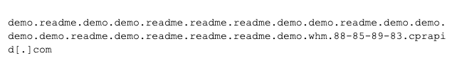
There were hundreds of others like that, all subdomains of
cprapid[.]com
. We suspect
cprapid[.]com
is what we would call a “wildcard” domain. That is, we think it’s configured to answer with a valid DNS response no matter what you ask it. Even if you were to mash the keyboard on your computer, and then end the query with
cprapid[.]com
, it would answer with an IP address. Normally, if you ask for a domain that doesn’t exist you would get a response of “No Such Domain” (aka NXDOMAIN). We think
cprapid[.]com
is configured to never do that. The reason we’re seeing that giant chain of crazy subdomains is because someone on the Internet has a dictionary of common subdomains, and is trying every possible combination…when they get an answer for a given subdomain, they recurse and try again on that subdomain. So, when a query to
demo.cprapid[.]com
succeeds, the script tries to discover subdomains of that, and tries
demo.demo.cprapid[.]com
, which succeeds, so it tries to find subdomains of
demo.demo.demo.cprapid[.]com
, and so on and so on.
Since we think none of those subdomains are ones the attacker bothered to configure, we will ignore it. We dropped any registrable domain that has more than 20 subdomains. If you see something like this, it’s probably worth mentioning to the researcher that you came across it, since wildcarding itself is interesting…but then drop it from further clustering efforts, since you can’t tell which ones are queries from people doing discovery on the net, and which ones are actual attacker actions.
Act Normal, Someone’s Coming
So, what patterns are in the subdomains? E.g. Do some of the registrable domains have the same set (or a similar set) of subdomains? That’s especially interesting if domains with the same subdomains are in different clusters from our last effort.
To test this, we pulled out all the subdomains, and made a mini “document” out of the words that make up the subdomains. This is similar to the clustering effort from an earlier webinar, but with a couple of twists:
- First, we will want to keep the registrable domain in the document, not for clustering purposes, but to make it clearer which domain we’re actually clustering. We want to prevent this from being used for clustering, however.
- Second, we will want to add a couple words to the “stop” words category, especially the subdomain “www.”
Sidebar – TF-IDF and stop words
We’re going to use a system called TF-IDF (Term Frequency-Inverse Document Frequency) for this part of the clustering. TF-IDF is a way of identifying the important or relatively unique words in a document when compared to a larger set of documents. For example, if you have a large set of news articles, the word “the” is probably in all of the documents. On the other hand, “rugby” probably wouldn’t occur often. So if “rugby” does appear, especially if it appears multiple times in one document, then TF-IDF would score it highly. Words that score highly in TF-IDF are a good indication of a word that’s important and unique to that document, and therefore a good indication that the word is meaningful for that document.
TF-IDF also has a notion of “stop words” — words so common you can’t infer meaning from them at all. “The” is a good example of a stop word as it appears globally across many or nearly all textual documents. In our case, we decided that we gained no special knowledge about a domain by learning that it had a subdomain of “www” so we added “www” as a stop word to the TF-IDF processing.
We would like to use TF-IDF here because we want to see if domains cluster together on the unusual subdomains that might be important to that particular domain, rather than common across all of them. For example, if it turns out that all the domains have a subdomain of “login”, that’s interesting, but we don’t want that to cause all the domains to cluster together into one big cluster. We would hope that “login” would score quite low in TF-IDF in that case, and any other subdomain words would drive the clustering instead.
In the end, we turned a list of domains like
[www.test.com, mail.test.com, secure.test.com, login.test.com]
into a single document like “
www mail secure login test.com.
” These documents went to DBSCAN after using TF-IDF to turn the documents into vectors like we did before). Before that, we did one last bit of cleanup: some domains had no subdomains, and others only had “www” as a subdomain. We removed all of those from this analysis.
Clustering worked well. It found some obvious clusters, like that all of the
scotlabank
impersonations had
scotlaonline
and auth subdomains. But, it also found some very interesting patterns around what appears to be attacker infrastructure. For example:

Those were all put into the same cluster. Notice that they’re quite different registrable domains, impersonating different banks, but they all share a fairly large set of words in their subdomains including “cpanel”. That’s the kind of detail that we would want to pass on to researchers, saying, “this cluster of seemingly unrelated registrable domains actually share something interesting in common…”
Epilogue
Human attention is a scarce resource, and as data volumes continue to grow it becomes even more challenging to find threats quickly. Clustering algorithms and text processing techniques can group domains together into an assumed impersonation target, and clustering over subdomains can possibly reveal threat actor behavior or other useful patterns.
We wanted to help threat researchers, especially to help them find information they might have trouble finding on their own, and to scale the analysis to larger and larger scales. All of the patterns we found were there in the data, but finding them manually can be tedious and error-prone. These techniques are a good way to speed investigations and help researchers find new, interesting, and actionable results faster.
Interested in clustering? You can download the Jupyter notebooks that implement all this here.
If you’re Interested in the world’s best domain and DNS data to power your own investigations, please reach out to us here!