Geolocating & Mapping IP Address Data From SIE


1. Introduction
As part of our effort to help people visualize data obtained from the Security Information Exchange (see the October 7th, 2016 post “Visualizing SIE Channel 204 Data”), we thought it might be interesting to try geolocating and mapping IP addresses from SIE Channel 204.
The IP addresses we’ll be working with are IP addresses for “sites that people are trying to access” (and NOT the IP addresses where queries are coming from NOR the IP addresses where SIE “sensor” or “collector” nodes are located).
2. Getting Some IP Address Data
We’ll begin by collecting five million observations from Channel 204 from an SIE blade server, saving those hits in JSON format into the file ch204-5000000.txt. We know that five million observations may sound like “a lot” to some of you, but it only takes five minutes or so of elapsed time to grab that data, as we can see from the following timestamps:
$ date ; nmsgtool -C ch204 -c 5000000 -J ch204-5000000.txt ; date
Tue Nov 29 19:16:00 UTC 2016
Tue Nov 29 19:21:11 UTC 2016
The output can be viewed with:
$ cat ch204-5000000.txt | jq '.' | less
[...]
{
  "time": "2016-11-29 19:15:28.399385850",
  "vname": "SIE",
  "mname": "dnsdedupe",
  "source": "[elided]",
  "message": {
    "type": "INSERTION",
    "count": 1,
    "time_first": "2016-11-29 19:14:54",
    "time_last": "2016-11-29 19:14:54",
    "response_ip": "[elided]",
    "bailiwick": "tumblr.com.",
    "rrname": "bilbypasadena.tumblr.com.",
    "rrclass": "IN",
    "rrtype": "A",
    "rrttl": 30,
    "rdata": [
      "66.6.32.21",
      "66.6.33.21",
      "66.6.33.149"
    ]
  }
}
Note that a single record may yield multiple IP addresses, as is the case for the example above (e.g., “66.6.32.21”,“66.6.33.21”, and “66.6.33.149”).
Other records may have NO IP address, as is the case for the following SOA (“Start of Authority”) record:
$ cat ch204-5000000.txt | jq '.' | less
[...]
{
  "time": "2016-11-29 19:15:51.064369203",
  "vname": "SIE",
  "mname": "dnsdedupe",
  "source": "[elided]",
  "message": {
    "type": "INSERTION",
    "count": 2,
    "time_first": "2016-11-29 10:46:27",
    "time_last": "2016-11-29 18:39:48",
    "response_ip": "[elided]",
    "bailiwick": "uniroyalchemical.com.",
    "rrname": "uniroyalchemical.com.",
    "rrclass": "IN",
    "rrtype": "SOA",
    "rrttl": 86400,
    "rdata": [
      "cbru.br.ns.els-gms.att.net. rm-hostmaster.ems.att.com. 13 83000 10000 600000 86400"
    ]
  }
}
We’ll be discarding any observations that don’t have an IP address (since without an IP address there’d be nothing to map).
3. Keeping Just Records That Have IP Addresses, and Stripping All Unneeded Text
Having retrieved and saved five million observations of the sort shown above, our next job is to strip away all the extraneous information from those records, leaving us with just a file of IP addresses which we can then geolocate. We use jq and grep (the regular Unix search command), to do that processing:
$ cat ch204-5000000.txt | jq -r .message.rdata[] | grep -v "\.$" | grep -v " " | grep -e "\." -e "\:" > sie-ips-5000000.txt
Decoding that command line (note that you may need to scroll to the right to see it all):
- cat ch204-5000000.txt streams our data for further processing.
- jq -r .message.rdata[] selects just the IP address field from the JSON format records; the -r asks that the field be written in “raw” form, without any formatting.
- grep -v “\.$” discards any records that end with a period. Records that end with a period are typically CNAME records or other records that do not contain an IP address.
- grep -v ” “ filters any records that include a blank (those are typically SOA records).
- grep -e “\.” -e “\:” filters any records that have neither a colon nor a period (all IP addresses will either have one or the other).
- The remaining output gets piped into the new file sie-ips-5000000.txt.
An aside: that file name may be a little misleading since in fact only 3,463,683 records remain after the filtering is finished:
$ wc -l sie-ips-5000000.txt
  3463683 sie-ips-5000000.txt
The IP addresses in that file look like:
$ less sie-ips-5000000.txt
207.192.72.221
176.9.47.11
195.110.124.188
178.77.214.22
184.168.221.22
2a01:4f8:150:6302::3
216.24.148.14
192.3.21.105
[etc]
Note that both IPv4 and IPv6 IP addresses may be present.
4. Geolocating IP Addresses Into Latitudes and Longitudes
To geolocate our IPs, we’ll use the terrific free geolocation data from IP2Location.[1]
You can see the small ip-to-lat-long.pl Perl script we used to resolve those IP’s to latitudes/longitudes in Appendix I, below.In order to be able to run the script, you’ll need:
- A copy of the Perl ip2location module
- A copy of the actual free geolocation databases
Running the little script is quite straight forward:
$ ./ip-to-lat-long.pl < sie-ips-5000000.txt > sie-ips-lat-long-5000000.txt
The resulting file looks like:
$ less sie-ips-lat-long-5000000.txt
40.735661, -74.172371
49.447781, 11.068330
43.766670, 11.250000
49.195221, 16.607960
33.601974, -111.887917
[etc]
5. Mapping the Data Points
We’re now ready to map the latitude and longitude data points.
For this program, we’re going to use the basemap matplotlib python toolkit,adapting an example that was formerly shared on the (sadly now-down)getdatajoy.com web site. You can find an archived copy here.
The required libraries and their documentation can be found here and here.
The small Python script is included below in Appendix II. Running it is also straight forward, requiring simply that we feed it a list of latitudes and longitudes, and list the starting and ending times for the title…
$ cat sie-ips-lat-long-5000000.txt | ./plot-sie-data-on-a-map.py 2016-11-29 19:16:00 2016-11-29 19:21:11
The resulting map gets shown on the user’s display, and in this case looks like:
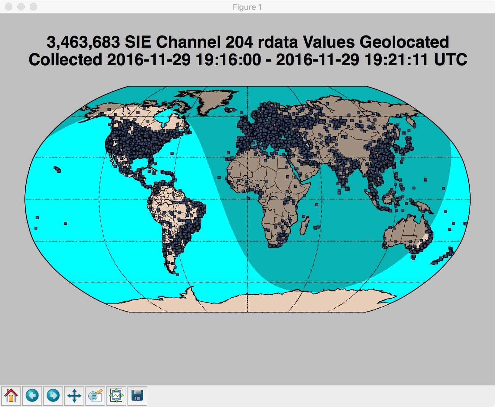
The grey sinusoidal region represents areas of the globe where the sun is down.
Dots on the map represent locations where there was an IP that mapped to that latitude and longitude.
As you might expect, North America, Europe and parts of the Far East appear to be particularly popular destinations.
Because of the number of points we’re plotting, the precise details are hard to make out in the densely-dotted regions, although if we zoom in 700% on a particular region (such as southeastern Australia), we can get a bit of a sense of how much overlap is occurring:

6. Creating a Heatmap?
More generally, this may be a perfect use case for employing a “heatmap” with the most densely visited regions being quite dark or “hot” and the less heavily visited being lighter.
Heatmaps are commonly seen today, with many built using Google Maps. Unfortunately, Google Maps can only work with a maximum of 10,000 points per map, while we need to map a “few more points” than that (roughly 3.5 million!) on our heatmap.
In part II of this series, we’ll describe how to use the free/open source QGIS as a more scalable alternative to create a heatmap for this data.
Joe St Sauver, Ph.D. is a Scientist for Farsight.
—Notes:
[1] This site or product includes IP2Location LITE data available from http://lite.ip2location.com.
https://www.ip2location.com/downloads/ip2location-perl-8.0.3.tar.gz
—
Appendix I. IP to Geolocation Script
#!/usr/bin/perl
use strict;
use warnings;
use Geo::IP2Location;
my $obj = Geo::IP2Location->open("IP2LOCATION-LITE-DB5.BIN");
my $obj2 = Geo::IP2Location->open("IP2LOCATION-LITE-DB5.IPV6.BIN");
my $input = <STDIN>;
my $latitude;
my $longitude;
if (index($input, ":") == -1)
  {
    $latitude = $obj->get_latitude($input);
    $longitude = $obj->get_longitude($input);
  }
  else
  {
    $latitude = $obj2->get_latitude($input);
    $longitude = $obj2->get_longitude($input);
  }

  print "( $latitude, $longitude )\n";
—
Appendix II. Plotting the geolocated points with Matplotlib
#!/usr/bin/env python

# adapted from the example that's at
# http://web.archive.org/web/20160803183440/https://www.getdatajoy.com/examples/python-plots/plot-data-points-on-a-map

import sys
import locale
import dateutil.parser
import numpy as np
import matplotlib.pyplot as plt
from mpl_toolkits.basemap import Basemap
from datetime import datetime

if len(sys.argv) == 1:
  print "Usage: ", sys.argv[0], "UTC_file_collection_START_time UTC_file_collection_STOP_time\ntime formats must be YYYY-MM-DD HH:mm:ss\n"
  sys.exit(2)
elif len(sys.argv) == 3:
  print "Must specify collection start AND stop times\n"
  print "For example: ", sys.argv[0], "2016-06-22 14:10:01 2016-06-22 14:45:01\n"
else:
  temptime1 = sys.argv[1] + " " + sys.argv[2]
  temptime2 = sys.argv[3] + " " + sys.argv[4]

siedata = np.genfromtxt(sys.stdin, delimiter=",",
   dtype=[('lat', np.float32), ('lon', np.float32)], usecols=(0, 1))

fig = plt.figure(figsize=(10, 7.5), dpi=80)
plt.subplots_adjust(left=0.05, right=0.95, bottom=0.1, top=0.9)

themap = Basemap( projection='robin', resolution = 'l',
   area_thresh = 100000.0, lon_0=0 )

themap.drawcoastlines()
themap.drawcountries()
themap.drawstates()
themap.drawparallels(np.arange(-90., 120., 30.))
themap.drawmeridians(np.arange(0., 360., 60.))

themap.fillcontinents(color = '#eacfb8')
themap.drawmapboundary(fill_color='aqua')

# mytime = datetime.utcnow()
mystarttime = dateutil.parser.parse(temptime1)
snooze = themap.nightshade(mystarttime, alpha=0.3)

x, y = themap(siedata['lon'], siedata['lat'])
themap.plot(x, y, 'o', color='#364866', markersize=4)

locale.setlocale(locale.LC_ALL, '')
mytemp0 = len(siedata)
mytemp1 = locale.format("%d", mytemp0, grouping = True)
mytemp2=mytemp1 + ' SIE Channel 204 rdata Values Geolocated\nCollected ' + temptime1 + ' - ' + temptime2 + ' UTC\n'

plt.title(mytemp2, fontsize=24, fontweight='bold')

plt.show()
Joe St Sauver, Ph.D. is a Scientist with Farsight Security, Inc.
Read more from DomainTools